Frequency Response Module

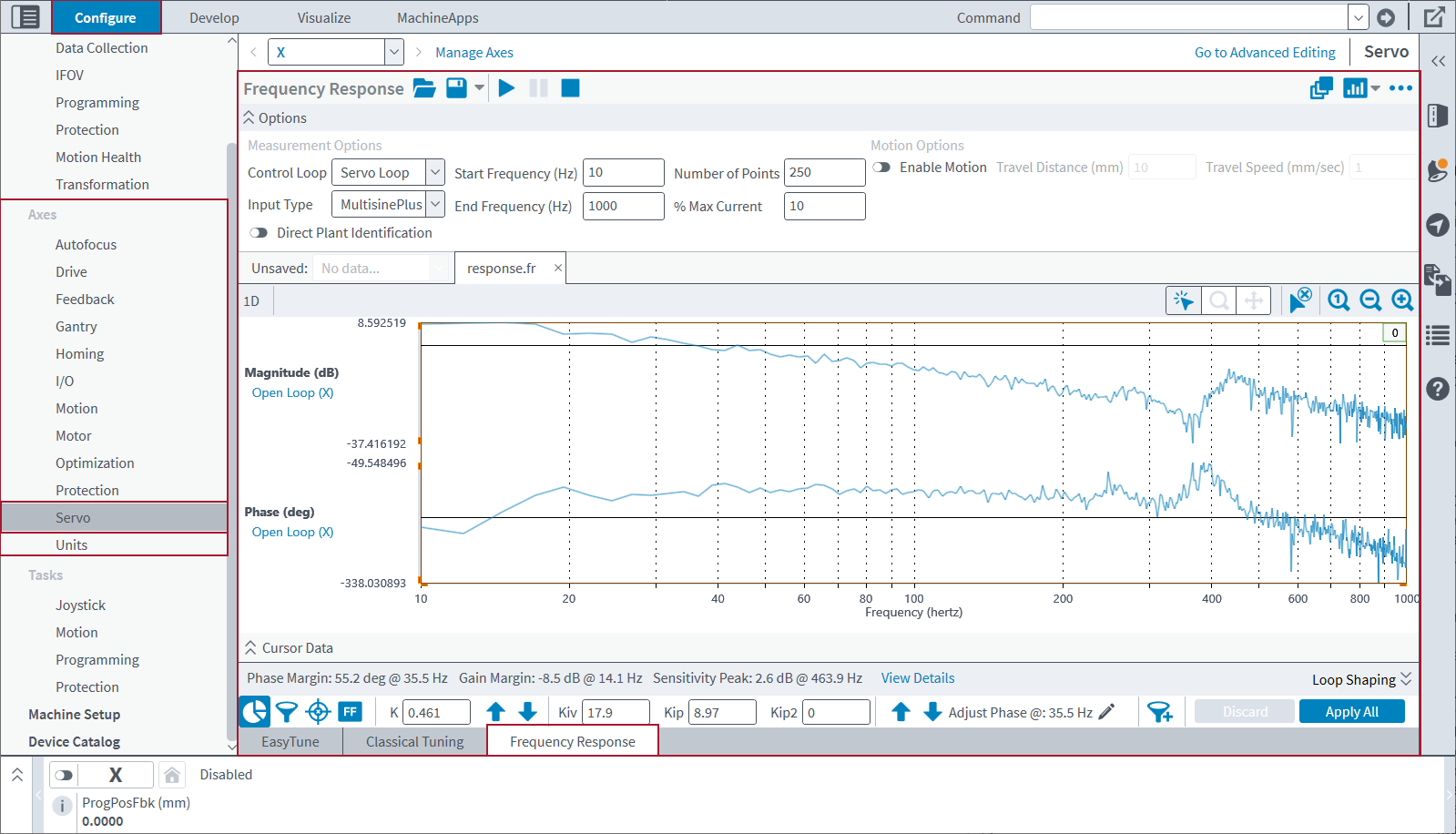
1. In the Axes category of Automation1 Studio, select the Servo topic. Then make sure that you are in the Basic Editing mode.
2. Select the Frequency Response module.
3. At the top of the module, click the drop-down arrow to select the axis that you want to configure.
4. In the Measurement Options toolbar, configure the Input Type, Start Frequency (Hz), End Frequency (Hz), frequency spacing, and the % Max Current. Based on the Input Type that you use, frequency spacing is the Number of Periods, Divisions, Averages, or Points.

Tip: Aerotech recommends that you the MultisinePlus input type.

How to use the MultisinePlus input type
1. The default values for MultisinePlus are 10 Hz for the Start Frequency (Hz) and 1000 Hz for the End Frequency (Hz). Make sure that the End Frequency (Hz) is less than or equal to half of the servo update frequency.
2. Start with the default amplitude that the application uses. If you find one or more points that are not valid in the final frequency response plot, you can increase the disturbance amplitude from the default value. The amplitude of the disturbance that is injected into the loop is shown in the application as one of the values that follow:
• A percentage of the maximum rated current of the controller, which is % Max Current.
• A percentage of the maximum rated voltage of the controller, which is % Max Voltage.
• A distance, which is Amplitude (mm).
5. If your axis has high friction or a coarse-resolution position encoder, toggle the Enable Motion slider to move the axis in the forward or reverse direction based on the motion parameters. Then configure the Travel Distance (primary units) and Travel Speed (primary units / second) in the Motion Options toolbar.
6. Click the Start Frequency Response Measurement button and wait for the measurement to complete.

The open-loop response type is almost always used to adjust and identify axis performance. The open-loop response is the response from a current command input at u_total to the feedback control effort output at u_c. It includes the Proportional-Integral-Derivative (PID) controller, the servo filters, and the plant. In Figure: Basic Controller Block Diagram, the open-loop response is the product of C*P. You can use the open-loop response to examine axis stability and dynamic performance. This response type also shows the phase margin, gain margin, crossover frequency, and low-end gain.

The plant response type is the response from a current command input at u_total to the position feedback output at y. It includes only the response of the stage and the current loop. After you measure a frequency response, the plant response is static. It does not change if you adjust the servo parameters. But if you change the value of the % Max Current and collect a new measurement, some conditions can cause the plant response to change. They are as follows:

• Your plant shows nonlinear behavior because of static friction in the bearings.
• Your plant shows nonlinear behavior because of Pulse-width modulation (PWM) dead-time in the drive.

The sensitivity response type is also used to adjust and identify axis performance. The sensitivity response is the response from a position command input at r to the position error output at e without feedforward compensation. This is equivalent to the response from a process disturbance at d to the feedback control effort at u_c. The sensitivity response identifies how the servo loop responds to disturbances, where a lower sensitivity magnitude makes the axis better at rejecting disturbances at that frequency. This response type also shows the sensitivity peak to make sure that the axis is stable.

The complementary sensitivity response is the response from a position command input at r to the position feedback output at y without feedforward compensation. If all of the feedforward gains are set to zero, the complementary sensitivity response is the same as the closed-loop response.

The process sensitivity response is the response from a disturbance at the plant input to the position feedback output at y. The process sensitivity response identifies the stiffness of the controlled system. It highlights frequency bands where the feedback controller can make the disturbances to the system larger in amplitude or make them smaller in amplitude.

The closed-loop response is the response from a position command input at r to the position feedback output at y, with feedforward compensation included. A closed-loop response that is near 0 dB magnitude and 0° phase is an indication of good tracking performance at that frequency.

The closed-loop error response is the response from a position command input at r to the position error output at e with feedforward compensation included. You can use the closed-loop error response to make an estimate of the magnitude of the tracking error at a specified frequency.

The Proportional-Integral-Derivative (PID) controller response is the response of the PID controller. It is calculated by the servo gain parameters.

The Proportional-Integral-Derivative (PID) controller and servo filters response is the response from a position error input at e to the feedback control effort at u_c.

The servo filters response is the response of the servo filters. It is calculated by the servo filter parameters.

The feedforward response is the response from a position command input at r to the feedforward control effort output at u_F. The inverse feedforward response is the response from an input at u_F to r. For the best dynamic performance, make sure that the magnitude and phase of the inverse feedforward response are almost the same as the plant response, where the plant response behaves almost the same as a free-mass model.

1. In the Axes category of Automation1 Studio, select the Servo topic. Then make sure that you are in Basic Editing mode.
2. Select the Frequency Response module.
3. At the top of the module, click the drop-down arrow to select the axis that you want to configure.
4. Select a target value for open-loop magnitude crossover frequency and the phase margin.

Tip: For information about applicable target values for a range of mechanical devices, refer to the Selecting a Maximum Target Crossover Frequency section of this guide. A phase margin in the range of 32 degrees to 45 degrees is permitted for most conditions.

5. On the top-right corner of the application, click the Plot Options button . On the Response Types menu, select Open Loop and Sensitivity.
6. On the bottom-left corner of the application, click the Edit servo loop filters button to change to the servo filter editing toolbar. When you adjust servo gains or servo filters in the frequency response editing toolbar, the Frequency Response module simulates the effects of the servo parameter changes without applying them to the axis.
7. Set the Cutoff Frequency of the Filter 00 - LowPass filter to a value that is 8 - 15x the target crossover frequency.
8. On the bottom-left corner of the application, click the Edit Servo Loop Gains button to change to the servo gain editing toolbar.
9. Click the magnitude loop-shaping arrows to adjust the open-loop magnitude until the shaped open-loop magnitude crossover frequency is the same as your target crossover frequency.
10. Use the phase loop-shaping arrows to adjust the reported phase margin until it is the same as your target phase margin.
11. If the reported sensitivity peak is above 6 dB or if the response shows encirclement, Aerotech recommends that you decrease your target crossover frequency. You can also increase the target phase margin if necessary. If the sensitivity peak or encirclement occurred because of a mechanical resonance, you can try to decrease the sensitivity peak with a servo filter. To do this, apply a notch filter at the resonant frequency to attenuate the open-loop magnitude.
12. To apply the servo parameter values to the controller, click the Apply button at the bottom of the application.
13. Do one more frequency response measurement. Then make sure that the Crossover Frequency, Phase Margin, and Sensitivity Peak are the same as the approximate values from the previous measurement.
14. When the performance of the selected axis is satisfactory, click the Save All button on the bottom-left corner of the application. This makes sure that the updated parameters will have an effect after the next controller reset.

The phase margin is the difference, in degrees, between the phase of the open-loop response at the magnitude crossover frequency and -180 degrees. In Figure: Margins and Axis Stability, the frequency at which the phase margin is calculated is highlighted with the red cursor.

The phase margin measures axis stability. It also measures robustness against variations in the plant dynamics. If you increase the phase margin, the axis becomes more stable. But if you decrease the phase margin, the axis becomes less stable and can stop being stable. If you specify a Phase Margin (deg) that is less than or equal to 20 degrees, it is possible that your axis will not be stable.

A larger phase margin gives you less oscillation and a better-damped response. But that response is slower. If the open-loop response has many magnitude crossover frequencies, then the overall phase margin is the worst and lowest phase margin across the system. If you specify a Phase Margin (deg) between 30 and 60 degrees, it balances performance and robustness satisfactorily.

The open-loop magnitude crossover frequency, which is also known as crossover frequency, is the frequency at which the magnitude of the open-loop response is zero dB. Here the open-loop gain is equal to one. The open-loop magnitude crossover frequency is used to calculate the phase margin. The first open-loop magnitude crossover frequency, where the magnitude initially moves from positive to negative values, is an indication of dynamic performance. Here a higher initial crossover frequency corresponds to a higher servo-loop bandwidth A measurement, expressed in frequency (hertz), of the range which an amplifier or motor can respond to an input command from DC to -3dB on a frequency sweep. and a faster rise time.

The gain margin is the gain in dB above or below the 0 dB line at the phase crossover frequency. If an open-loop response has many phase crossover frequencies, then the gain margin is the worst and lowest absolute value of all the gain margins. In Figure: Margins and Axis Stability, the frequency at which the gain margin is calculated is highlighted with the purple cursor.

A low absolute value for the gain margin usually causes high-frequency noise and robustness that is not sufficient to variations in load. If you specify a gain margin of 8 dB, it balances performance and robustness satisfactorily.

The sensitivity peak shows the maximum amplitude of the sensitivity response. The sensitivity peak does not always occur at the same frequency as the phase margin or gain margin. It shows the worst stability margin across all frequencies. In Figure: Margins and Axis Stability, the sensitivity peak occurs at 121 Hz, between the open-loop magnitude crossover and the higher-frequency open-loop phase crossover.

You can use the magnitude of the sensitivity response to measure how stable the axis is. When you do this, larger magnitudes cause the axis to be less stable at that frequency. The axis will be stable if the peak of the sensitivity curve is less than or equal to 6 dB and the response does not show encirclement. The phase of the sensitivity response is not related to how stable the axis is.