6.2. Interpolation
Aerotech recommends that you do not measure a high-density grid (for example, 65 x 65 points = 4,225 marks). This process uses a large quantity of time and data. A better method is to mark and measure a Coarse grid, such as 5 x 5 or 9 x 9. Then, interpolate the intermediate points to make a high-density correction table.
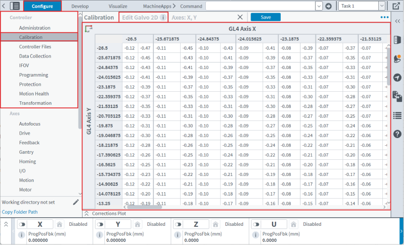
How to interpolate a calibration table in Automation1 Studio
- Collect Coarse Data: Measure a sparse 9 x 9 grid across the full Field of View (FOV).
- Load Data: In Automation1 Studio, manually create a calibration table. Use 9 x 9 for the Sample Distances. For instructions on how to do this, refer to
- Edit Properties: Select the table that you created. Click the Menu (...) button. Then select Edit File Properties. A dialog comes into view where you can edit the properties of the selected table.
- Rescale: In the Edit File Properties dialog, change the Sample Counts for the X and Y axes to the maximum possible density. For example, you might increase this from 9 to 65.
- Execute: Click OK to commit your changes and close the dialog. Automation1 Studio automatically applies bi-cubic interpolation to calculate the correction values for the new intermediate points. Then the system fills the 65 x 65 grid between your initial 9 x 9 measurements.
IMPORTANT: Aerotech recommends that you interpolate calibration tables to the maximum permitted size. For example, 65 x 65 for the GI4 or a maximum of 138,000 points for the GL4. High-density tables decrease the step size of corrections between grid points. This makes smoother motion and decreases quantization errors during high-speed scanning. The bi-cubic interpolation method usually matches the error patterns caused by F-Theta lenses. It also gives you accurate estimates of correction values when you interpolate between measured points.